One of many major outcomes of our paper is the introduction of a mathematical framework, that permits governments to evaluate the comfort to intervene with bailout investments in distressed banks’ fairness and optimise their choices. Within the following subsections, we first current the community mannequin of economic establishments, its dynamics and contagion mechanism, after which suggest an MDP based mostly on the community, which might be used to mannequin authorities interventions on bailed-out monetary establishments. After formulating the issue, we proceed with a technique for fixing the MDP and a few of the mathematical technicalities. Lastly, we implement our framework and methodology on two case research and current our findings.
Community of economic establishments
We think about a community whose set ({{{{{{{mathcal{I}}}}}}}}={1,ldots,N}) of nodes represents monetary establishments. Every node (iin {{{{{{{mathcal{I}}}}}}}}) is characterised at time t by a likelihood of default PDi(t)∈(0,1) per time interval Δt, a complete asset Wi(t) and an fairness Ei(t), that’s the capital utilized by node i as a buffer to face up to monetary losses, satisfying Ei(t) ≤ Wi(t).
The sting (i, j) of the community represents the publicity of node i to the default of node j the place (i,ne, jin {{{{{{{mathcal{I}}}}}}}}). Every edge (i, j) is related to a numerical worth wij which is dependent upon the contagion channels thought-about. For instance, we will think about solely credit score exposures or additionally the influence as a result of hearth gross sales of frequent belongings. Concerning credit score exposures, a lot of the instances solely aggregated values can be found, e.g. the full quantity of inter-banking belongings and liabilities for every node, and in such circumstances, bespoke algorithms are used to deduce the community of bilateral exposures (see, e.g. refs. 37, 42). To consider authorities interventions aimed toward limiting the general losses, we use an adaptation of the PD mannequin launched in ref. 37 by extending it to permit the likelihood for the nodes to incur additionally optimistic shocks, by way of investments within the nodes, reasonably than simply destructive shocks because of the default of different nodes. The main target of this paper can also be radically completely different from the one in ref. 37, which focuses on the losses sustained by personal buyers, since we’re right here solely within the losses incurred by the taxpayers. Within the following, we are going to measure the time in discrete time steps which might be multiples of Δt, i.e. t + 1 is equal to t + Δt.
We outline the full influence Ii(t) on node i at time t, because of the default of different nodes (jin {{{{{{{mathcal{I}}}}}}}}setminus {i}) within the community and their publicity wij, by
$${I}_{i}(t): !!=mathop{sum}limits_{jin {{{{{{{mathcal{I}}}}}}}}setminus {i}}{w}_{ij}{delta }_{j}(t),quad ,{{mbox{for all}}},iin {{{{{{{mathcal{I}}}}}}}},$$
(1)
the place
$${delta }_{j}(t)=left{start{array}{l}1,quad ,{{mbox{if node}}},,j,{{mbox{defaults at time}}},,t, 0,quad {{{{{{{rm{in any other case}}}}}}}}.hfill finish{array}proper.$$
The mechanism by which defaults will happen at every time step t, yielding δ⋅(t) = 1, might be constructed in the direction of the top of this part utilizing all community data, together with the probabilistic framework as much as time t. The influence Ii(t) represents a loss for the full asset Wi, which in flip decreases additionally the fairness Ei of node i, therefore decreasing their worth at time t + 1. This may be seen from the accounting equation for every node i, specifically
$${W}_{i}(t)={E}_{i}(t)+{B}_{i}(t),$$
(2)
which states that the full asset Wi is all the time equal, always, to the fairness Ei plus the full legal responsibility Bi. Be aware that Bi isn’t affected by the losses as it’s comprised of loans from different banks, deposits, and so forth., which might be due in full except the financial institution i defaults. Therefore, we’ve got
$$Delta {W}_{i}(t)=Delta {E}_{i}(t),$$
(3)
the place we outline ΔXi(t) ≔ Xi(t + 1)−Xi(t). Taking into consideration additionally the potential improve ΔJi(t) within the cumulative funding Ji(t) of the federal government in node i as much as time t, which can in flip improve the values of the full asset Wi and fairness Ei of node i at time t + 1, we will write
$${W}_{i}(t+1)={W}_{i}(t)-{I}_{i}(t)+Delta {J}_{i}(t)qquad {{{{{{{rm{and}}}}}}}}qquad {E}_{i}(t+1)={E}_{i}(t)-{I}_{i}(t)+Delta {J}_{i}(t).$$
(4)
The likelihood of default PDi(t) of node i is elevated by the influence Ii(t) at time t, since a part of the capital buffer (fairness Ei) is misplaced, and decreased by the potential funding ΔJi(t), which in flip grows the capital buffer. With a purpose to mannequin the impact of the influence Ii(t) and potential funding ΔJi(t) on PDi(t), we use right here the credit score danger mannequin launched by Merton38. Alternatively, it’s attainable to make use of the primary passage mannequin launched by Black and Cox43. The implied likelihood of default PDM is subsequently calculated as a operate of the parameters of every node:
$$PDM(W,E,mu,sigma ): !!=1-Phi left(left(log frac{W}{W-E}+mu -frac{{sigma }^{2}}{2}proper)bigg/sigma proper),$$
(5)
the place the time period W−E represents the full legal responsibility B of every financial institution, Φ is the univariate normal Gaussian distribution, μ is the drift (anticipated progress fee) and σ is the volatility of the geometric Brownian movement related to the full asset W within the Merton mannequin. We then use (5) to acquire the likelihood of default of node i,
$$P{D}_{i}(t):!=max left{PDM({W}_{i}(t),{E}_{i}(t),{mu }_{i},{sigma }_{i}),PD{M}_{i}^{,,flooring}proper},$$
(6)
the place we introduce the mounted quantity (PD{M}_{i}^{flooring}), whose goal is to exclude unreasonably low chances of default, basically appearing as a decrease certain of the PDi. A decrease certain (PD{M}_{i}^{flooring}) is important, as regardless of how properly a financial institution i is capitalised towards losses, it will possibly nonetheless default as a result of excessive occasions equivalent to pure disasters, political revolutions, sovereign defaults, and so forth. With out (PD{M}_{i}^{flooring}), the federal government would underestimate the precise likelihood of default and would have a tendency to take a position extra capital than it’s handy. For example of calibration of this parameter, we will comply with the usual assumption that the PDi of a financial institution (iin {{{{{{{mathcal{I}}}}}}}}) is bigger or equal to the likelihood of default of the nation the place it’s based mostly in. On this context, the (PD{M}_{i}^{flooring}) can be the likelihood of the nation internet hosting financial institution i to default on its debt.
Now, if node i loses an quantity of capital Ii(t) larger than its capital buffer (fairness Ei(t)), at a while t, the full asset Wi(t) turns into lower than its legal responsibility Bi(t) and it’s handy for the shareholders to train their choice to default. In apply, when this happens, we set PDi(t + 1) = 1 and node i’ll default at time t + 1. Furthermore, recall that node i might also default at any time t with likelihood PDi(t) as a result of its personal particular person traits given by (6); see additionally the default mechanism described on the finish of this subsection
Now, when node i defaults, we denote by LGDi the loss given default of node i, which is a set quantity representing the share of the cumulative investments Ji on node i by the federal government, that can’t be recovered after a default. In case of default of node i, we additional assume that along with the aforementioned lack of investments, the taxpayers’ loss Li can also be comprised of a set share αi (for comfort) of the full asset Wi of the node i. That’s, the taxpayers’ total loss Li(t) at time t is given by
$${L}_{i}(t):!!!={alpha }_{i}{W}_{i}(t)+LG{D}_{i},{J}_{i}(t).$$
(7)
To finish our framework, we have to specify the likelihood of a couple of default taking place throughout the identical time step, given the PDi of every node i obtained as in (6). For instance, if the nodes had been unbiased, the likelihood of nodes i and j defaulting on the identical time step, denoted by PD[ij], can be the product of the person chances PDi and PDj. On this paper, we enable nodes to depend upon one another and use a Gaussian latent variable mannequin (see, e.g. ref. 44) to calculate the possibilities of simultaneous defaults of two or extra nodes. To be extra exact, the likelihood of a finite subset of nodes ({i,j,okay,ldots }subseteq {{{{{{{mathcal{I}}}}}}}}) of the community defaulting on the identical time, is given by
$$P{D}_{[i,, j,k,ldots ]}: !!={int}_{D}{Phi }_{N}^{prime}({{{{{{{bf{u}}}}}}}};Sigma )d{{{{{{{bf{u}}}}}}}},$$
(8)
the place ({Phi }_{N}^{prime}) is the standardised multivariate Gaussian density operate, with zero imply and a symmetric correlation matrix Σ ∈ [−1, 1]N×N, given by
$${Phi }_{N}^{prime}({{{{{{{bf{u}}}}}}}};Sigma ): !!=frac{exp {-frac{1}{2}{{{{{{{{bf{u}}}}}}}}}^{T}{Sigma }^{-1}{{{{{{{bf{u}}}}}}}}}}{sqrt{{(2pi )}^{n},|Sigma|}}$$
(9)
and ∣Σ∣ is the determinant of Σ. We additional notice that the combination area D in (8) is the Cartesian product of the intervals ([-infty,{Phi }_{1}^{-1}(P{D}_{l})]) for every node l that belongs to the set of defaulting nodes {i, j, okay,…}, and the intervals [−∞,∞] for the remaining non-defaulting nodes, the place ({Phi_{1}}) is the univariate normal Gaussian distribution.
We at the moment are able to current the mechanism in response to which nodes can default based mostly on their particular person traits. To be extra exact, at every time step t, we first pattern values (x1,…,xN) of the random vector (X={({X}_{1},{X}_{2},ldots,{X}_{N})}) with the multivariate Gaussian distribution of the underlying Gaussian latent variable mannequin talked about above. Then, we assume that node i defaults in response to the rule:
$${x}_{i}, < ,{Phi }_{1}^{-1}(P{D}_{i}(t))quad iff quad {delta }_{i}(t)=1.$$
(10)
The banks bailout downside as a Markov Determination Course of
On this subsection, we describe the federal government choices of bailing out banks as a Markov Determination Course of (MDP) pushed by our framework described within the earlier subsection. We firstly assume that the federal government estimated that the disaster will seemingly be over at time M, the place every time step could possibly be interpreted to mirror the contagion impact, which happens throughout durations in our mannequin, or the governmental overview frequency of the likelihood to spend money on monetary establishments within the midst of a disaster. In any case, recalling that the federal government invests within the fairness of banks and different monetary establishments, we assume that will probably be in a position to promote the acquired shares to the personal sector, after the top of the disaster, for a worth that’s much like the buying one. In actuality, this worth is straight linked to the expectation of the long run dividends to be paid by the surviving financial institution. The federal government may then realise a revenue on these investments, after a substantial rise within the mixture inventory market on the finish of the disaster, from time M + 1 onwards (see ref. 45 for a related analysis investigation), and even make a loss. Clearly, any situation would have an effect on the efficient taxpayers loss. On this paper although, we focus solely on the minimisation of taxpayers losses as a result of bailouts and financial institution defaults throughout the disaster episode (time Zero to M), by assuming a impartial realised return on investments in surviving establishments past time M.
We outline the 4-tuple (S, As, Pa, Ra) of the set S of all of the states of the dynamic community (specifically the state area wherein the processes’ evolution takes place, resulting in all attainable configurations of the monetary system), set As of all actions accessible to the federal government from state s ∈ S, transition chances ({P}_{a}(s,{s}^{prime})=P({s}_{t+1}={s}^{prime},|,{s}_{t}=s,{a}_{t}=a)) between state s at any time t and state ({s}^{prime}) at time t + 1 having taken motion a ∈ As at time t, and rewards ({R}_{a}(s,{s}^{prime})) (destructive losses in our mannequin) acquired after taking motion a at any time t whereas being at state s and touchdown in state ({s}^{prime}) at time t + 1, the place (s,{s}^{prime}in S). Moreover, we think about a continuing low cost issue γ with 0 ≤ γ < 1, in order that rewards obtained sooner are extra related. The discounted cumulative reward G from time step t till the top of disaster (recall {that a} full episode consists of M time steps) is subsequently outlined by
$$G(t): !!!=mathop{sum }limits_{u=t}^{M-1}{gamma }^{u-t}{R}_{{a}_{u}}({s}_{u},{s}_{u+1}^{prime}).$$
(11)
Within the remaining of this subsection, we increase on the 4-tuple (S, As,Pa,Ra) that defines our MDP and formulate our stochastic management downside.
Firstly, we introduce the MDP states. The states st ∈ S, at every time t, wherein the monetary system could find yourself, are outlined by three major pillars: (a) all of the parameters of the community (Wi(t), Ei(t), PDi(t), Ji(t), LGDi, αi, μi, σi, wij, Σij, for i, j ∈ {1,…,N}, the place wii = 0), (b) an listed set ({{{{{{{{mathcal{I}}}}}}}}}_{def}(t)subseteq {{{{{{{mathcal{I}}}}}}}}) containing all defaulted nodes previous to time t and (c) the time to maturity M−t.
Secondly, we introduce the MDP actions and governmental insurance policies. The MDP actions ({a}_{t}in {A}_{{s}_{t}}) in our mannequin are the management variables of the federal government when making an attempt to minimise the losses of the community (i.e. maximise the anticipated G in (11)). They correspond to injections of capital ({a}_{t}to {{{{{{{boldsymbol{Delta }}}}}}}}{{{{{{{{bf{J}}}}}}}}}^{{{{{{{{bf{a}}}}}}}}}(t): !!=(Delta {J}_{1}^{a}(t),Delta {J}_{2}^{a}(t),ldots,Delta {J}_{N}^{a}(t))) growing the federal government’s investments within the nodes (1, 2,…,N), affecting their complete wealth and fairness in response to (4), whose up to date (elevated) values are denoted by
$${J}_{i}^{a}(t): !!={J}_{i}(t)+Delta {J}_{i}^{a}(t),quad {W}_{i}^{a}(t): !!={W}_{i}(t)+Delta {J}_{i}^{a}(t)quad {{{{{{{rm{and}}}}}}}}quad {E}_{i}^{a}(t): !!={E}_{i}(t)+Delta {J}_{i}^{a}(t).$$
(12)
These extra assets on one hand, make the nodes extra resilient, therefore diminishing their up to date likelihood of default (P{D}_{i}^{a}) by way of (5), (6), specifically
$$P{D}_{i}^{a}(t): !!!=max {PDM({W}_{i}^{{a}}(t),,{E}_{i}^{a}(t),,{mu }_{i},,{sigma }_{i}),,PD{M}_{i}^{flooring}},$$
(13)
resulting in (statistically) much less defaults because of the up to date default mechanism (recall (10)) given by
$${x}_{i}, < ,{Phi }_{1}^{-1}left(P{D}_{i}^{a}(t)proper)quad iff quad {delta }_{i}^{a}(t)=1,$$
(14)
and consequently to an up to date (statistically decreased) complete influence
$${I}_{i}^{a}(t): !!=mathop{sum}limits_{jin {{{{{{{mathcal{I}}}}}}}}setminus {i}}{w}_{ij}{delta }_{j}^{a}(t),quad ,{{mbox{for all}}},,iin {{{{{{{mathcal{I}}}}}}}}.$$
(15)
Alternatively, these assets might be in danger in case of node i defaulting at time t, for the reason that aforementioned (elevated) cumulative funding ({J}_{i}^{a}) and complete wealth ({W}_{i}^{a}) will each contribute in the direction of an elevated up to date taxpayers’ total loss ({L}_{i}^{a}) given by way of (7) by
$${L}_{i}^{a}(t): !!={alpha }_{i}{W}_{i}^{a}(t)+LG{D}_{i},{J}_{i}^{a}(t).$$
(16)
Recalling that every motion ({a}_{t}in {A}_{{s}_{t}}) is dependent upon the present state st at any time t, we denote the federal government coverage by a operate π(st) → at that signifies which motion to take at every state. A coverage that minimises the anticipated community losses known as optimum coverage and is denoted by π*, whereas the motion ({a}_{t}^{*}) returned by π* given a state st (i.e. ({pi }_{*}({s}_{t})to {a}_{t}^{*})) is then referred to as the optimum motion for that state.
Be aware that, the mannequin can simply incorporate additionally the character of governmental fairness injections (asking banks to repay debt, or spend money on safer belongings to hedge towards future losses, or change their technique in alternate for funding), that will ultimately result in up to date ({mu }_{i}^{a}(t)={mu }_{i}(Delta {J}_{i}^{a}(t))) and ({sigma }_{i}^{a}(t)={sigma }_{i}(Delta {J}_{i}^{a}(t))) affecting solely the ensuing up to date likelihood of default (P{D}_{i}^{a}(t)) in (13), whereas the remainder of our framework and methodology would stay intact.
Thirdly, we introduce the MDP transition chances. Inside our framework, a node that has defaulted doesn’t contribute to future losses and can’t turn out to be lively once more, i.e. the cardinality of the set of defaulted nodes (|{{{{{{{{mathcal{I}}}}}}}}}_{def}(t)|) is a non-decreasing operate of time t. Therefore the transition likelihood ({P}_{a}(s,{s}^{prime})) from state ({s}) to ({s}^{prime}) might be non-zero just for states ({s}^{prime}) that: (a) have the identical quantity or extra defaulted nodes than state s; (b) are “reachable”, within the sense that their traits PDi(t + 1), Wi(t + 1) and Ei(t + 1), for (iin {{{{{{{mathcal{I}}}}}}}}setminus {{{{{{{{mathcal{I}}}}}}}}}_{def}(t+1)) (the remaining lively nodes in ({s}^{prime})) take values which might be coherent with eqs. (4)–(6) after calculating the impacts Ii(t) from the newly defaulted nodes (iin {{{{{{{{mathcal{I}}}}}}}}}_{def}(t+1)setminus {{{{{{{{mathcal{I}}}}}}}}}_{def}(t)) at time t. For an instance on establish these so-called reachable states, we consult with the Reachable MDP states instance within the Strategies part.
Then, for all states ({s}_{t+1}^{prime}) with a non-zero transition likelihood ({P}_{{a}_{t}}({s}_{t},{s}_{t+1}^{prime})), we will calculate the latter by way of the Gaussian latent variable mannequin (see additionally (8), (9)). To be extra exact, given the federal government investments relative to motion at at state st and time t, we use the up to date ({J}_{i}^{a}(t),{W}_{i}^{a}(t),{E}_{i}^{a}(t)) and (P{D}_{i}^{a}(t)) from (12)–(13) to calculate the transition likelihood by way of (see additionally (8)) the next integral:
$${P}_{{a}_{t}}({s}_{t},{s}_{t+1}^{prime}): !!={int}_{D}{Phi }_{|{{{{{{{mathcal{I}}}}}}}}setminus {{{{{{{{mathcal{I}}}}}}}}}_{def}(t)|}^{prime}({{{{{{{bf{u}}}}}}}};{Sigma }_{sub}(t))d{{{{{{{bf{u}}}}}}}},$$
(17)
the place ({Phi }^{prime}) is the density given by (9) with dimension equal to the cardinality of the set of surviving nodes (|{{{{{{{mathcal{I}}}}}}}}setminus {{{{{{{{mathcal{I}}}}}}}}}_{def}(t)|le N). Upon recalling the up to date model of the default mechanism in (14), the combination area D in (17) is given by the Cartesian product of the intervals ([-infty,{Phi }_{1}^{-1}(P{D}_{i}^{a})]) for the extra defaulted nodes (iin {{{{{{{{mathcal{I}}}}}}}}}_{def}(t+1)setminus {{{{{{{{mathcal{I}}}}}}}}}_{def}(t)) and the intervals ([{Phi }_{1}^{-1}(P{D}_{i}^{a}),infty ]) for all of the remaining lively nodes (iin {{{{{{{mathcal{I}}}}}}}}setminus {{{{{{{{mathcal{I}}}}}}}}}_{def}(t+1)) at state ({s}_{t+1}^{prime}). The Σsub(t) is the sub-matrix of the unique correlation matrix Σ after eradicating the rows and the columns equivalent to defaulted nodes (iin {{{{{{{{mathcal{I}}}}}}}}}_{def}(t)) at state st.
Thus, we observe that in our mannequin, the transition chances rely solely on the federal government investments at, the ensuing monetary establishments’ likelihood of default (P{D}_{i}^{a}) and the correlation construction Σij with (i,,jin {{{{{{{mathcal{I}}}}}}}}setminus {{{{{{{{mathcal{I}}}}}}}}}_{def}(t)) which hyperlinks the monetary establishments within the community.
Fourthly, we introduce the MDP rewards. In our mannequin the rewards take non-positive values, since their total maximisation has to translate for our MDP into the minimisation of the potential total taxpayers’ losses ({L}_{i}^{a}(t)) in (16) for all nodes (iin {{{{{{{mathcal{I}}}}}}}}setminus {{{{{{{{mathcal{I}}}}}}}}}_{def}(t)) after taking motion at at every time t. Particularly, in gentle of the up to date default mechanism (14), we outline the reward at time t by
$${R}_{{a}_{t}}({s}_{t},{s}_{t+1}^{prime}): !!=-mathop{sum}limits_{iin {{{{{{{mathcal{I}}}}}}}}setminus {{{{{{{{mathcal{I}}}}}}}}}_{def}(t)}left({alpha }_{i}{W}_{i}^{a}(t)+LG{D}_{i},{J}_{i}^{a}(t)proper){delta }_{i}^{a}(t),$$
(18)
the place solely the nodes defaulting at time t after taking motion at, i.e. having ({delta }_{i}^{a}(t)=1), contribute to the sum of losses. Which means that the reward at time t might be 0, in case there are not any extra defaults occurring at time t.
Lastly, we’re able to outline the optimum worth operate and current the stochastic management downside formulation. By doing so, we are going to formalise the principle intention of the federal government, which is the minimisation of taxpayers’ losses throughout the disaster episode. We subsequently want our mannequin to point if the federal government ought to intervene and if that’s the case, which quantity it ought to make investments for a given configuration of the monetary system to realize its aforementioned objective. This mathematically interprets to the federal government aiming at discovering the optimum actions ({a}_{t}^{*}in {A}_{{s}_{t}}), or equivalently the optimum coverage π*, for successive time steps, ranging from any time t and any attainable state st of the dynamic community till the top of the episode at time M, in an effort to maximise the anticipated discounted cumulative reward G(t) given by (11).
The optimum worth operate V*(st) is then outlined because the anticipated discounted cumulative reward G(t) ranging from state st at time t and following the aforementioned optimum coverage π*, given in gentle of the definition of rewards (particularly their expression in (18)) by
$${V}_{*}({s}_{t}): ! ={E}_{{pi }_{*}}[G(t)|{s}_{t}]={E}_{{pi }_{*}}left[mathop{sum }limits_{u=t}^{M-1}{gamma }^{u-t}{R}_{{a}_{u}}({s}_{u},{s}_{u+1}^{prime}) bigg| {s}_{t}right] =-{E}_{{pi }_{*}}left[mathop{sum }limits_{u=t}^{M-1}{gamma }^{u-t}mathop{sum}limits_{iin {{{{{{{mathcal{I}}}}}}}}setminus {{{{{{{{mathcal{I}}}}}}}}}_{def}(u)}left({alpha }_{i}{W}_{i}^{a}(u)+LG{D}_{i},{J}_{i}^{a}(u)right){delta }_{i}^{a}(u)bigg| ,{s}_{t}right] forall quad t,in [0,M-1]quad {{{{{{{rm{and}}}}}}}}quad {V}_{*}({s}_{M}): !!=0,$$
(19)
the place the latter definition follows because of the time step M signifying the top of the disaster episode, when the federal government can promote all its shares within the banks, thus incurring no extra losses.
Given the definition of π*, the optimum worth operate V*(st) represents the utmost anticipated discounted cumulative reward, which interprets into the minimal anticipated discounted taxpayers’ loss, that may be obtained amongst all attainable insurance policies π ranging from st,
$${V}_{*}({s}_{t}) =mathop{max }limits_{pi }{E}_{pi }[G(t)|{s}_{t}] =-mathop{min }limits_{pi }{E}_{pi }left[left.mathop{sum }limits_{u=t}^{M-1}{gamma }^{u-t}mathop{sum}limits_{iin {{{{{{{mathcal{I}}}}}}}}setminus {{{{{{{{mathcal{I}}}}}}}}}_{def}(u)}left({alpha }_{i}{W}_{i}^{a}(u)+LG{D}_{i}{J}_{i}^{a}(u)right){delta }_{i}^{a}(u)right|{s}_{t}right].$$
(20)
The optimum motion worth operate Q*(st, at) is the anticipated discounted cumulative reward we get hold of, if we first take motion at whereas being at state st after which comply with the optimum coverage π* for any of the successive steps from t + 1 till the top of the episode M. Mathematically, that is outlined by
$${Q}_{*}({s}_{t},{a}_{t}): ={E}_{{pi }_{*}}[G(t)|{s}_{t},{a}_{t}] =Eleft[left.{R}_{{a}_{t}}({s}_{t},{s}_{t+1}^{prime})right|{s}_{t},{a}_{t}right]+{E}_{{pi }_{*}}left[left.mathop{sum }limits_{u=t+1}^{M-1}{gamma }^{u-t}{R}_{{a}_{u}}({s}_{u}^{prime},{s}_{u+1}^{prime})right|{s}_{t},{a}_{t}right].$$
(21)
Equally to the optimum worth operate, Q*(st, at) represents the utmost anticipated cumulative reward that may be obtained when ranging from st and after taking motion at at time t.
The contribution of the optimum motion worth operate in offering the specified quantitative analysis required for implementing the mannequin in real-life situations is twofold. Firstly, discover that discovering Q* is equal to fixing the MDP, for the reason that optimum motion ({a}_{t}^{*}) for every state st (therefore the optimum coverage π*) might be obtained by
$${a}_{t}^{*}=mathop{{{{{{{{rm{argmax}}}}}}}}}limits_{{a}_{t}},{Q}_{*}({s}_{t},{a}_{t}).$$
(22)
Secondly, we use Q* in an effort to quantify the comfort to intervene Conv(st) for the federal government at every state st and any time t, within the forthcoming mannequin implementations. To be extra exact, we outline by Conv(st) the distinction between the optimum motion worth operate equivalent to the very best governmental intervention and the optimum motion worth operate related to ({a}_{t}^{0}), which denotes the inaction (no investments) at time t, when being on the state st, i.e.
$${{{{{{{rm{Conv}}}}}}}}({s}_{t}): !!=mathop{max }limits_{{a}_{t}in {A}_{{s}_{t}}setminus {{a}_{t}^{0}}}{{Q}_{*}({s}_{t},{a}_{t})}-{Q}_{*}({s}_{t},{a}_{t}^{0}).$$
(23)
AI method to resolve the MDP
On this subsection, we current our synthetic intelligence method to resolve the MDP, pushed by our dynamic community of the monetary system that may be managed by a regulator in view of minimising the anticipated taxpayers’ loss.
We firstly recall a typical relationship between optimum worth features and motion worth features in MDPs. Observe that the 2 phrases on the right-hand aspect within the definition (21) of the optimum motion worth operate Q*(st, at) are first the instant anticipated reward at time t as a result of taking motion at and second the optimum anticipated discounted cumulative reward from time t + 1 onwards. We will subsequently rewrite Q*(st,at) from (21) when it comes to the transition chances (recall (17)) and the long run optimum worth features ({V}_{*}({s}_{t+1}^{prime})) outlined in (19), within the kind
$${Q}_{*}({s}_{t},{a}_{t})=mathop{sum}limits_{{s}_{t+1}^{prime}}{P}_{{a}_{t}}({s}_{t},{s}_{t+1}^{prime})({R}_{{a}_{t}}({s}_{t},{s}_{t+1}^{prime})+gamma {V}_{*}({s}_{t+1}^{prime})).$$
(24)
It is usually simple to see from the definitions (19) and (21) of the optimum worth operate V*(st) and motion worth operate Q*(st,at), respectively, that
$${V}_{*}({s}_{t})=mathop{max }limits_{{a}_{t}},{Q}_{*}({s}_{t},{a}_{t}),$$
(25)
i.e. the utmost anticipated discounted cumulative reward from st is the one equivalent to the utmost worth of Q* amongst all accessible potential actions ({a}_{t}in {A}_{{s}_{t}}) at time t. Substituting the expression of (24) in (25) thus offers the Bellman optimality equation
$${V}_{*}({s}_{t})=mathop{max }limits_{{a}_{t}in {A}_{{s}_{t}}}left{mathop{sum}limits_{{s}_{t+1}^{prime}}{P}_{{a}_{t}}left({s}_{t},{s}_{t+1}^{prime}proper)left({R}_{{a}_{t}}left({s}_{t},{s}_{t+1}^{prime}proper)+gamma {V}_{*}left({s}_{t+1}^{prime}proper)proper)proper}.$$
(26)
On condition that we’ve got an entire description of our MDP (particularly, we’ve got the transition chances ({P}_{{a}_{t}}({s}_{t},{s}_{t+1}^{prime})) and the rewards ({R}_{{a}_{t}}({s}_{t},{s}_{t+1}^{prime}))), we may in concept enumerate all attainable states, use Dynamic Programming and the Worth Iteration algorithm (see ref. 46) to resolve our stochastic management downside. This might basically contain discovering V* utilizing the Bellman optimality equation in (26) after which calculating Q* by way of (24), thus fixing the MDP. Nevertheless, making use of this normal concept isn’t a scalable/possible method as a result of (a) the complexity of the MDP states and (b) the large variety of successor states ({s}^{prime}) (for all however trivial networks), making normal computations not possible.
We, subsequently, suggest on this paper an method to resolve the MDP, which includes the usage of a variation of the Fitted Worth Iteration algorithm (see, e.g. refs. 40, 41) with bespoke traits uniquely constructed in our synthetic intelligence method.
Our methodology consists of the next 4 steps:
-
(i)
Devise a parametric illustration ({overline{V}}_{*}(s,beta )) for the optimum worth operate V*(s), the place β is a placeholder for a set of parameters to suit (see our building within the Worth operate approximation subsection, Strategies part);
-
(ii)
Use ({overline{V}}_{*}(s,beta )) to plan a parametric illustration ({overline{Q}}_{*}(s,a,beta )) for the optimum motion worth operate Q*(s, a) in (24) (see the Motion worth operate approximation subsection, Strategies part, for its derivation and our method to calculate it);
-
(iii)
Use ({overline{Q}}_{*}(s,a,beta )) for the right-hand aspect of (25) to acquire an approximate Bellman optimality equation in an effort to match β by way of a studying course of (see our method within the Studying course of subsection, Strategies part), which can ultimately give ({V}_{*}(s),approx ,{overline{V}}_{*}(s,{beta }^{;match}));
-
(iv)
Lastly, use ({overline{V}}_{*}(s,{beta }^{;match})) to calculate ({overline{Q}}_{*}(s,a,{beta }^{;match}),approx ,{Q}_{*}(s,a)), and therefore clear up the MDP as within the Optimum answer of the MDP subsection, Strategies part.
Every one of many aforementioned steps bares its personal difficulties and technical obstacles, which we overcome within the evaluation introduced within the aforementioned subsections of the Strategies part.
Within the following subsections, we use our synthetic intelligence method to resolve the MDP in two implementation case research. We present how our mannequin works and procure qualitative outcomes on the optimum bailout resolution downside confronted by governments. An expert calibration of our mannequin would require the trouble and firepower of a central financial institution or a authorities workplace, and entry to delicate information. Nonetheless, by exploring these two case research, we offer helpful insights for whether or not and when taxpayers ought to fund financial institution bailouts.
Setup of implementation case research
As an example how our methodology works and its potential, we apply our mannequin on each an artificial homogeneous community (Krackhardt kite graph) and an actual community of the European world systemically necessary establishments. Earlier than we current our case research, we assign values to a set of parameters, which might be frequent to each case research (except in any other case specified). We think about a disaster episode that can final for M = 7 time steps, a reduction issue γ = 0.98 and an preliminary authorities funding Ji(0) = Zero for every node (financial institution or different monetary establishment) (iin {{{{{{{mathcal{I}}}}}}}}). Furthermore, we assume the odds αi of wealth loss upon default of node i to be all the identical, i.e. αi = α, and we conservatively assume that the anticipated worth of the full wealth’s return is μi = 0, for all (iin {{{{{{{mathcal{I}}}}}}}}). Recall that, we’re contemplating fairness investments by the federal government that may be recovered, in case of default, solely after all of the depositors and bond holders are glad. Therefore, we assume that the federal government loses all its investments in case of default, i.e. LGDi = 1, for all (iin {{{{{{{mathcal{I}}}}}}}}). If the federal government is allowed to make use of different means in addition to fairness investments, e.g. bond investments, then LGDi ∈ (0, 1) (see ref. 47 for a research on senior and subordinated restoration charges). Nevertheless, this is able to suggest a softer impact on the solvency points and require a modification of the likelihood of default system in (13), for the reason that funding wouldn’t be straight affecting the fairness (12) anymore. With a purpose to consider the typical correlation between monetary establishments, we use a homogeneous correlation matrix for our nodes, which is about to Σij = 0.5 for (ine j,in ,{{{{{{{mathcal{I}}}}}}}}setminus {{{{{{{{mathcal{I}}}}}}}}}_{def}) following ref. 48. The volatility σi of the full wealth’s return for every (iin {{{{{{{mathcal{I}}}}}}}}), is calculated at time Zero by inverting (5) utilizing the preliminary (recognized) values of PDi(0), Ei(0) and Wi(0). The values of σi, (iin {{{{{{{mathcal{I}}}}}}}}), are then assumed to stay fixed at successive time steps of the simulation, from time 1 to M. Lastly, we set the ground of the likelihood of default for every node i as (PD{M}_{i}^{flooring}=0.00021), which is the higher finish of the AAA default likelihood bracket inside the inner credit standing methodology utilized by Credit score Suisse49. Within the sequel, we denote the accessible governmental funding actions by
$$ < {{{{{{{rm{node}}}}}}}} > ,@ , < ,{{mbox{capital investment as a tenth of a percent of the total asset}}},W > ,$$
with the conference that an motion that considers all nodes is indicated with
The frequent theme is that including exterior assets makes the community extra resilient, however such assets might be misplaced in a subsequent default, which creates a trade-off for the decision-maker. The optimum coverage that balances this trade-off and minimises the general anticipated taxpayers’ loss is an optimum answer to our MDP, and is analysed within the forthcoming two research.
Case research 1: KK community
This research considerations a community with homogeneous nodes organised because the Krackhardt kite (KK) graph (Fig. 1, see additionally ref. 50), which is known as the KK community. The principle cause for selecting the KK graph as an underlying community is to primarily assess whether or not our algorithm can distinguish between central nodes and peripheral ones. Particularly, we use the community traits when it comes to the centrality of nodes 4, Eight and 10 (see Fig. 1), to research how bailout choices depend upon the nodes’ place within the community. Nevertheless, we may even examine extra hypotheses and attain necessary monetary conclusions on bailout resolution making.
Fig. 1: Krackhardt Kite (KK) community.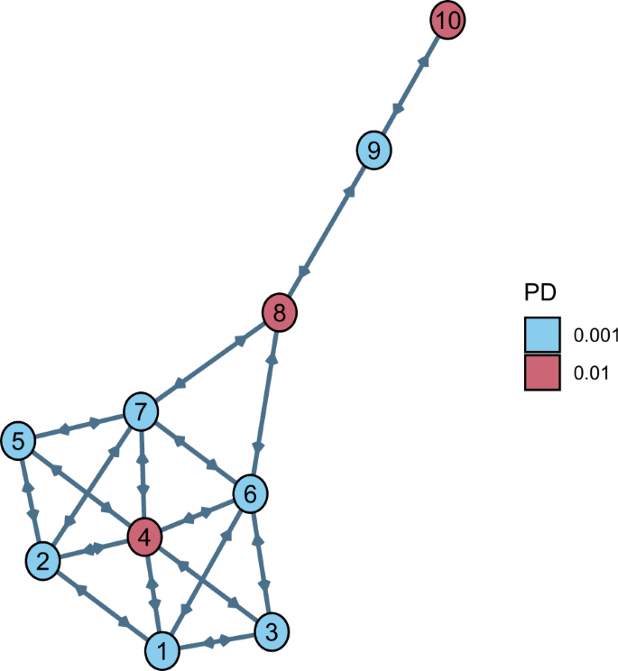
The KK community is used to evaluate how bailout choices are influenced by node centrality. The ten nodes of the graph in ({{{{{{{mathcal{I}}}}}}}}={1,ldots,10}) signify monetary establishments, that are similar aside from their chances of default (PD) at time 0, that are PDi(0) = 0.01, for i ∈ {4, 8, 10}, and PDi(0) = 0.001, for (iin {{{{{{{mathcal{I}}}}}}}}setminus {4,8,10}). All of them have a normalised complete asset Wi(0) = 100 and capital Ei(0) = 3. The perimeters between nodes, representing claims between monetary establishments, are oriented and homogeneous, assuming the worth wij = 1, for all (i,ne, jin {{{{{{{mathcal{I}}}}}}}}).
On this case research, all of the nodes (banks or different monetary establishments) have complete asset Wi(0) = 100 and capital Ei(0) = 3. As proven in Fig. 1, the nodes in crimson color have likelihood of default PDi(0) = 0.01, for i ∈ {4, 8, 10}, whereas the others have PDi(0) = 0.001, for (iin {{{{{{{mathcal{I}}}}}}}}setminus {4,8,10}). The perimeters between nodes are oriented and homogeneous, assuming the worth wij = 1, for all (i ,ne, jin {{{{{{{mathcal{I}}}}}}}}). For the sake of this case research, we prohibit the potential funding quantities in every node i to be: 0, 0.5% Wi, 1% Wi, 1.5% Wi or 2% Wi. Moreover, the federal government can select at every time step to spend money on the one nodes 4, 8, 10 or in all nodes.
The optimum motion worth operate Q*(s0, a0) at time Zero is illustrated in Fig. 2 for 3 situations of percentages of wealth loss upon default. Particularly, for a “comparatively low” α = 0.0001, the very best motion (minimising losses) is to not spend money on any financial institution (0@0). Transferring from the highest to the underside panel (as α will increase) the choice to not make investments turns into an increasing number of expensive to the system. For a “comparatively intermediate” α = 0.001, not investing is roughly equally beneficial to investments in single monetary establishments, whereas for a “comparatively excessive” α = 0.01, the very best motion turns into to take a position 1.5% Wi in all monetary establishments (0@15). It is usually attention-grabbing to notice that (see Fig. 2) no matter the α-value: (i) investing the utmost quantity of two% Wi in all banks (0@20) is rarely your best option; (ii) offering the minimal capital (0@05) is all the time the worst alternative, as the extra funding is just too small to make them resilient, however nonetheless will increase the funds in danger in case of default. The sensitivity of the optimum coverage with respect to α might be additional examined in additional element additionally in our subsequent (extra life like) case research.
Fig. 2: Optimum motion worth operate Q* for the Krackhardt Kite (KK) community.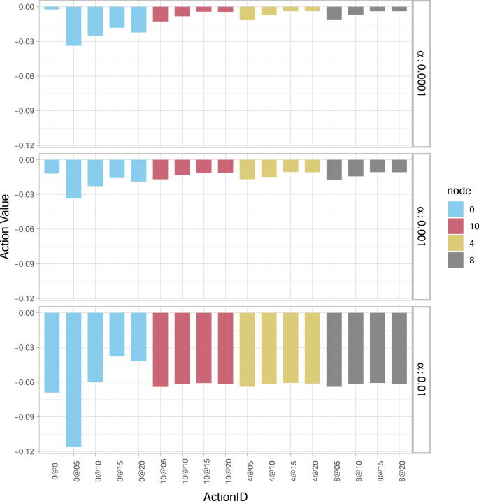
The optimum motion worth operate Q*(s0, a0) at time Zero for various actions a0 (a authorities funding of 0, 0.5, 1, 1.5 or 2 within the fairness of the nodes) and values of share wealth loss upon default α (0.0001, 0.001 and 0.01). Within the legend, the colors establish the nodes {0, 10, 4, 8} within the determine (Zero represents all nodes). On the x axis, the ActionID 0@Zero means no funding, 0@05 means investing 0.5 in all of the nodes, 10@05 means investing 0.5 in node 10, and so forth. For a small worth of α = 0.0001, the very best motion is to not make investments (0@0). As α will increase, so does the comfort of investing extra capital. For α = 0.01 the very best motion (equivalent to smallest loss) is to take a position 1.5 in all of the nodes (0@15). It’s by no means handy to take a position the utmost quantity of capital (0@20), whereas investing 0.5 in all of the nodes (0@05) is the worst motion for all values of α, as the extra capital isn’t sufficient to strengthen the community and it’s in danger following potential defaults.
Fixing the share of wealth loss upon default at α = 0.0001, we now focus our evaluation on the central node 4, representing a monetary establishment with a number of hyperlinks and interconnections with its friends, versus the peripheral node 10, representing a comparatively remoted monetary establishment linked solely with one different (see Fig. 1). The leads to Fig. 3a conclude that investing within the central node Four is all the time higher than within the peripheral node 10 for a similar quantity of capital and all such decisions. Thus, our algorithm certainly reveals a transparent choice in central reasonably than peripheral node investments.
Fig. 3: Optimum motion worth operate Q* for the Krackhardt Kite (KK) community as a operate of time to the top of disaster.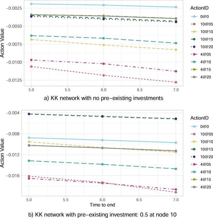
The outcomes are obtained for the share α = 0.0001 of wealth loss upon default, and concentrate on nodes 4 (central node) and 10 (peripheral node). Within the legend, the ActionID 0@Zero means no funding, 0@05 means investing 0.5 in all of the nodes, 10@05 means investing 0.5 in node 10, and so forth. a The algorithm feels the community construction and suggests to spend money on node 4 (resulting in smaller loss) reasonably than node 10. b In case the federal government had beforehand invested in node 10, the federal government wants to guard its funding by optimally risking a further funding in node 10.
Nevertheless, the outcomes change when the federal government had already invested even the minimal attainable quantity of 0.5% W10 within the peripheral node 10. On this case, Fig. 3b with J10(0) = 0.5 concludes {that a} substantial extra funding in financial institution 10 (specifically, 10@15 or 10@20) largely outperforms every other technique—together with not investing in any respect, and all sorts of investments within the central node 4. Such a consequence signifies that the optimum technique for the federal government is subsequently to maintain investing (sufficiently excessive quantities of capital) in node 10, aiming at saving this already invested capital J10(0) = 0.5. This governmental tendency to supply capital to distressed banks if that they had already invested in them creates ethical hazard, because the financial institution may act haphazardly counting on the implicit authorities assure. The truth that bailouts create ethical hazard has been emphasised extensively within the monetary and financial literature, each theoretically and empirically (see e.g., refs. 51,52,53,54). Furthermore, on condition that the assumed J10(0) = 0.5 is the worst amongst all attainable investments in a single node at time 0 (see each Fig. 2 and Fig. 3a), the instructed optimum, extra, considerably massive funding within the peripheral node 10, could possibly be additionally seen as an eventual strengthening of the initially weak funding of 0.5% W10.
Lastly, we carry out a sensitivity evaluation of the optimum motion versus the period of disaster. Regardless of the kind of funding, the leads to Fig. 3a present that the optimum motion worth operate Q* decreases in absolute worth (i.e. measurement of losses decreases) because the time to the top of the episode M−t decreases. The principle cause is that every node of the community is unstable with an related likelihood of default per unit time, therefore the shorter the time horizon the decrease the anticipated losses. Moreover, the contagion has much less time to propagate, which explains additionally why the node’s place within the community turns into much less and fewer related.
Case research 2: EBA community
After having thought-about a small artificial graph within the first case research, we now research a community of the European world systemically necessary establishments (GSII, see Desk 1) obtained from the info offered by the European Banking Authority55, which is known as the EBA community. Be aware that, the unique information don’t include the whole bilateral community of exposures, as that is thought-about business-sensitive data. Whereas the particular publicity between two banks is unknown, the aggregated credit score publicity of a financial institution versus different monetary establishments is offered. For every financial institution i within the set ({{{{{{{mathcal{I}}}}}}}}) of the European GSII, we’ve got its complete inter-bank asset ({sum }_{jin {{{{{{{mathcal{I}}}}}}}}}{w}_{ij}) and legal responsibility ({sum }_{jin {{{{{{{mathcal{I}}}}}}}}}{w}_{ji}), which can be utilized to reconstruct a community that satisfies the constrains (see, e.g. algorithms described in refs. 37, 42). The reconstructed community (see Fig. 4) might be completely different however has comparable traits to the precise community of bilateral exposures. The values of complete asset Wi(0) and capital Ei(0) at time Zero used for every monetary establishment i are reported in Desk 1. The possibilities of default are derived utilizing information from the credit standing company Fitch56 and present that the nodes with the upper likelihood of default are Monte dei Paschi di Siena (MPS) and BFA (see each Desk 1 and Fig. 4).
Desk 1 European Union’s World Systemically Vital Establishments (GSII)Fig. 4: Most spanning tree of the European Banking Authority (EBA) community.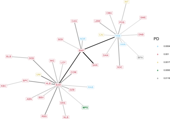
The community of the European Union’s World Systemically Vital Establishments (GSII) has been reconstructed from aggregated information accessible on the EBA web site55. Every node represents a monetary establishment (see Desk 1), its color represents its likelihood of default (PD), and darker edges establish stronger exposures.
To facilitate our evaluation, we firstly fake that the European Union (together with the UK) is a fiscal union with a single regulator (“authorities”) that’s accountable to all European taxpayers. Then, we think about any particular person states’ investments in banks previous to 2014 as “personal” investments, therefore we set the preliminary regulator investments to be Ji(0) = Zero for all (iin {{{{{{{mathcal{I}}}}}}}}). For the sake of this case research, we prohibit the potential funding quantities to inject in every monetary establishment i to be: 0, 0.5% Wi, 1% Wi, 1.5% Wi, 2% Wi, 2.5% Wi or 3% Wi. Moreover, we assume that the federal government can select at every time step t to spend money on all of the nodes which might be thought-about “dangerous” at the moment, outlined as every monetary establishment (iin {{{{{{{mathcal{I}}}}}}}}setminus {{{{{{{{mathcal{I}}}}}}}}}_{def}) with PDi > 0.009, in response to our (arbitrarily) chosen threshold. On this case research, the notation 0@05 thus signifies an funding of 0.5% Wi in every dangerous node (iin {{{{{{{mathcal{I}}}}}}}}setminus {{{{{{{{mathcal{I}}}}}}}}}_{def}).
For an in depth quantitative and qualitative evaluation, we depend on the comfort measure Conv for the federal government, outlined in (23), to intervene with fairness investments and we analyse the system for 4 completely different percentages α ∈ {0.0001, 0.001, 0.005, 0.01} of wealth loss upon default. We observe from Fig. 5a that, we’ve got a comfort Conv > Zero for increased percentages of wealth loss upon default (α = 0.01, 0.005 and 0.001), thus investing is a beneficial motion, whereas Conv < Zero for smaller α (α = 0.0001), implying that it isn't handy for the federal government to take a position. That is in line with our first case research utilizing the KK community (earlier subsection), as investing an quantity of capital is handy just for comparatively excessive values of α, in an effort to make the community sufficiently resilient.
Fig. 5: The comfort to intervene Conv for the European Banking Authority (EBA) community as a operate of time to the top of disaster.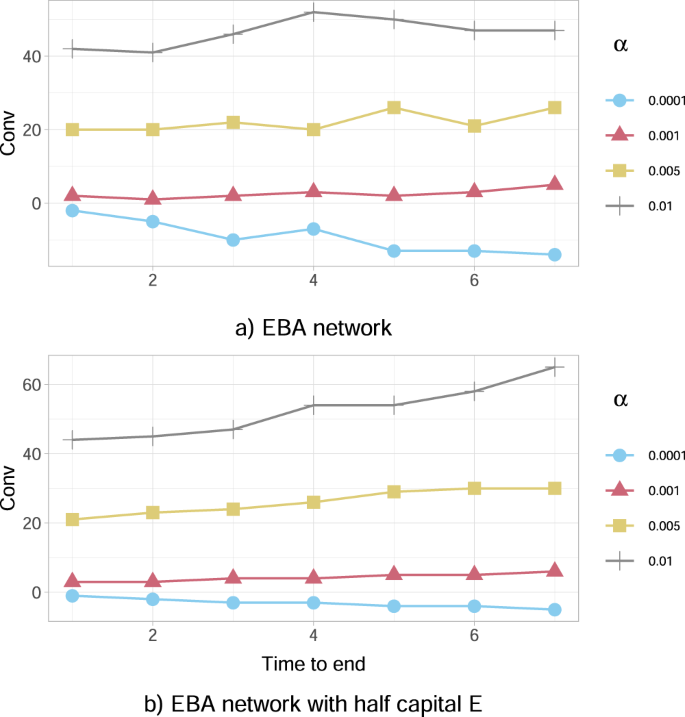
a The Conv (in tens of millions of EUR) outlined in (23) is optimistic for increased percentages of wealth loss upon default (α = 0.01, 0.005, 0.001), thus investing is a beneficial motion. Conversely, Conv < Zero for smaller α (α = 0.0001), implying that it isn't handy for the federal government to take a position. Conv tends to be an growing operate of the time to the top of the disaster when optimistic, and a reducing operate when destructive. b A severely distressed model of the community, the place the banks' capital Ei(0) has been artificially halved (all different traits are the identical). We observe that such a misery has the impact of accelerating Conv for every worth of α.
A sensitivity evaluation of the comfort to intervene for the federal government is additional examined versus the period of disaster, the preliminary capital and the credit score exposures of economic establishments:
-
(a)
The leads to Fig. 5a additional conclude that the comfort to intervene tends to be an growing operate of the time to the top of the episode M−t when Conv > Zero and a reducing operate when Conv < 0. This suggests that the comfort to intervene or not, weakens (decreases in absolute worth) as we method the top of the disaster. Apparently although, it seems that the character of the motion doesn't change with time, for the reason that operate Conv doesn't change signal.
-
(b)
Our leads to Fig. 5b additional present that the comfort to intervene Conv depends on the banks’ resilience, expressed by way of the preliminary capital Ei(0) of every financial institution i. Particularly, this severely distressed model of the community, the place the worth of Ei(0) has been artificially halved in contrast with the unique case research introduced in Fig. 5a, has the impact of accelerating the comfort Conv for the federal government to intervene for every worth of α. A extra thorough evaluation in Fig. 6a additional reveals that the comfort to intervene will increase on common because the monetary establishments’ preliminary capital Ei(0) decreases, for all period lengths of the disaster. It’s attention-grabbing to additionally notice that, this comfort intensifies considerably for bigger lengths of time till the top of the disaster.
Fig. 6: The comfort to intervene Conv for the European Banking Authority (EBA) community as a operate of the time till the top of disaster.
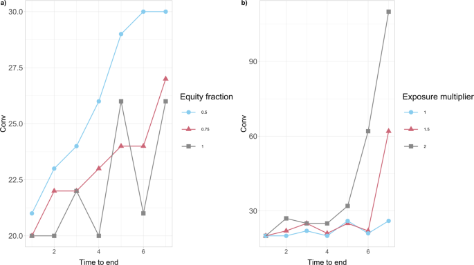
The values of Conv (in tens of millions of EUR) are obtained for the share α = 0.005 of wealth loss upon default. a We think about completely different percentages (50%, 75%, 100%) of the preliminary capital Ei(0) accessible to monetary establishments i at time 0. Conv tends to extend on common because the monetary establishments’ preliminary capital Ei(0) decreases. It is usually attention-grabbing to notice that, this comfort intensifies for bigger lengths of time till the top of the disaster. b We think about completely different multipliers (1, 1.5, 2) of the bilateral credit score exposures wij of economic establishments i to the default of j at time 0. Conv will increase because the wij’s improve and the influence of longer disaster period on Conv is very large.
-
(c)
It is usually clear from the leads to Fig. 6b that the comfort to intervene will increase because the bilateral credit score exposures wij between monetary establishments throughout the entire community improve. It’s attention-grabbing to additional observe that the influence of longer disaster period on the comfort to intervene is very large.
A sensitivity evaluation of the governmental optimum motion can also be examined versus the low cost issue, the monetary establishments’ chances of default and credit score exposures, the share of wealth loss upon default and the preliminary capital:
-
(a)
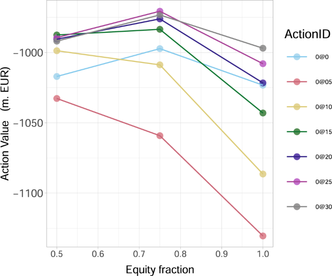
Our evaluation in Fig. 7a reveals clearly that the optimum motion worth operate Q*(s0, a0) at time Zero decreases for all potential actions because the low cost issue γ will increase. That’s, as the long run losses turn out to be extra related (from the governmental perspective), the anticipated systemic losses improve in absolute worth, whereas the optimum motion doesn’t change qualitatively.
Fig. 7: The optimum motion worth Q*(s0, a0) for the European Banking Authority (EBA) community at time 0.
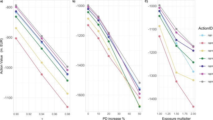
Within the legend, ActionID 0@Zero means no funding, 0@05 means investing 0.5 in all of the nodes, and so forth. The outcomes are obtained for the share α = 0.005 of wealth loss upon default. a As a operate of low cost issue γ, Q*(s0, a0) decreases, for all potential actions a0, as γ will increase. b As a operate of the share improve of the possibilities of default PDi(0) of economic establishments i at time 0, Q*(s0, a0) decreases, for all potential actions a0, as PDi(0) improve. c As a operate of the magnitude of multiplier of the bilateral credit score exposures wij of economic establishments i to the default of j, Q*(s0, a0) decreases, for all potential actions a0, as wij improve.
-
(b)
Our leads to Fig. 7b then present that the optimum motion worth operate Q*(s0,a0) at time Zero decreases (taxpayers’ losses improve in absolute worth) for all potential actions, with growing chances of default. Two attention-grabbing options showing are: (i) the initially narrowly optimum motion (0@30) turns into clearly optimum as the possibilities of default improve; (ii) the worst attainable motion, specifically the one to keep away from, modifications from the smallest attainable funding of 0.5percentWi to bigger investments of 1.0percentWi, 1.5percentWi in all dangerous monetary establishments i. That’s, even these medium measurement extra investments usually are not sufficient to make them resilient, however nonetheless considerably improve the funds in danger in case of default.
-
(c)
Our leads to Fig. 7c additionally present that the optimum motion worth operate Q*(s0, a0) at time Zero decreases for all potential actions, with growing bilateral credit score exposures wij between monetary establishments throughout the entire community. We additionally notice that the distinction within the efficiency of the optimum funding of a giant quantity (0@30) and non investing in any respect, will increase with larger credit score exposures amongst establishments.
-
(d)
It has already been confirmed by each case research into consideration (KK and EBA community subsections), that as the share α of potential wealth loss upon default will increase, the inaction (no investments) turns into much less handy for the federal government. We now intention to discover additional the transition between the situations when it’s handy and never handy for a regulator to intervene, by finding out the optimum motion values Q*(s0, a0) at time Zero with respect to modifications in α. Our leads to Fig. 8a conclude that: (i) there exists a vital αc ≈ 0.00079 that splits the parameter area of α-values into two “wealth loss regimes” of excessive/low values, reflecting governmental motion/inaction, respectively; (ii) the optimum motion at time Zero modifications drastically (non-smoothly) from a don’t make investments something coverage for α just under αc to an make investments the utmost quantity of three.0percentWi in all dangerous establishments i (0@30) coverage for α simply above αc. Discover that, these actions are in truth the 2 extremes. That is an attention-grabbing consequence as one might need anticipated a smoother transition between optimum actions as α will increase.
Fig. 8: The optimum motion worth Q*(s0, a0) for the European Banking Authority (EBA) community at time Zero as a operate of the share α of wealth loss upon default.
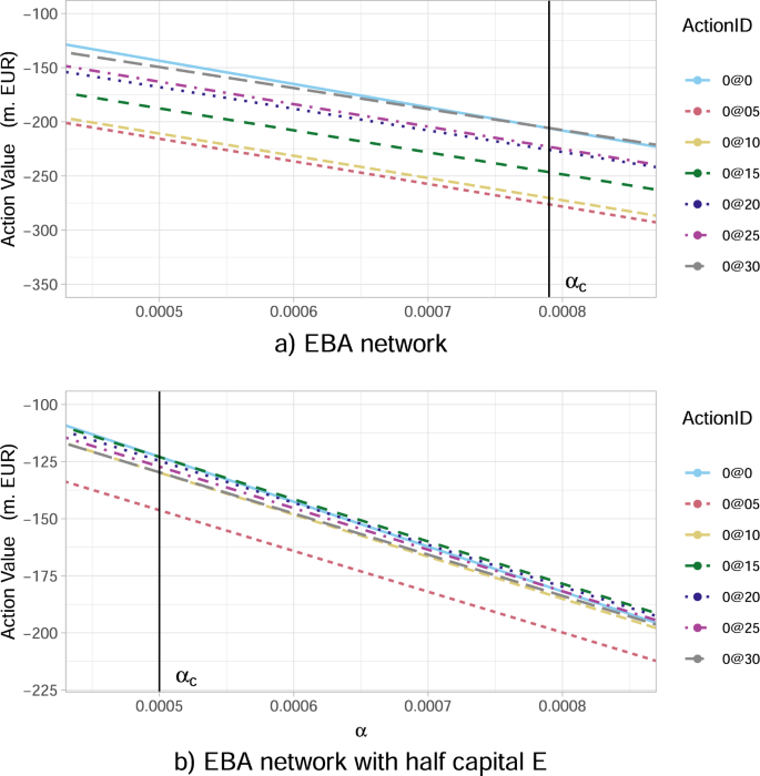
Within the legend, the ActionID 0@Zero means no funding, 0@05 means investing 0.5 in all of the nodes, and so forth. a There’s a vital worth of α given by αc ≈ 0.00079, past which the inaction of the federal government is not optimum. Particularly, for α simply above the vital αc, the very best motion turns into the funding of three.0percentWi in all dangerous monetary establishments i (0@30). b A severely distressed model of the community, the place the banks’ capital Ei(0) has been artificially halved (all different traits are the identical). We observe that such a misery impacts Q*(s0, a0) at time Zero and the worth αc at which a regulatory intervention turns into beneficial is decrease, specifically αc ≈ 0.0005. The optimum motion turns into the funding of 1.5% Wi in all dangerous monetary establishments i (0@15).
-
(e)
We then conclude from our leads to Fig. 8b, which is a severely distressed model of the unique community (introduced in Fig. 8a), the place the monetary establishment i’s capital Ei(0) has been artificially halved, that the optimum motion worth operate Q*(s0, a0) at time Zero modifications considerably each quantitatively and qualitatively. Apparently, the optimum motion for α > αc turns into the significantly decreased funding of 1.5% Wi in all dangerous monetary establishments i (0@15), in comparison with the unique community (see Fig. 8a). A extra thorough evaluation in Fig. 9 reveals that, because the preliminary capital Ei(0) decreases, the optimum funding quantity certainly decreases as properly. Particularly, we observe that the funding of three.0percentWi in all dangerous monetary establishments i, turns into 2.5percentWi when the capital decreases by 25% and 1.5percentWi when the capital decreases by 50%. Moreover, our leads to Fig. 9 reveal that the universally (for all Ei(0)) worst motion is to take a position the decrease quantity of 0.5percentWi in all dangerous monetary establishments i, as such a further funding is just too small to make them resilient, however nonetheless will increase the funds in danger in case of default.
Fig. 9: The optimum motion worth Q*(s0, a0) for the European Banking Authority (EBA) community at time Zero as a operate of the share of preliminary capital Ei(0) accessible to monetary establishments i.
Within the legend, the ActionID 0@Zero means no funding, 0@05 means investing 0.5 in all of the nodes, and so forth. The outcomes are obtained for the share α = 0.005 of wealth loss upon default and present that the very best motion a* amongst a0’s (equivalent to the best Q*(s0, a0) worth) decreases (0@30 → 0@25 → 0@15) as Ei(0) lower.
Lastly, we carry out a sensitivity evaluation of the aforementioned wealth loss regimes versus the monetary establishments’ preliminary capital. We will conclude from our leads to Fig. 8b that, because the monetary establishment i’s capital Ei(0) decreases, the worth αc separating the 2 wealth loss regimes of unfavourable and beneficial regulatory interventions, is considerably decrease αc ≈ 0.0005. Particularly, the federal government is keen to intervene for a lot decrease percentages of wealth loss.